End-to-end QP-based policies:
A unified perspective on robust control and robot learning

Fausto Vega1, Priyanka Supraja Balaji2, Chase Dunaway1, Joe Koszut1,
Jon Arrizabalaga1, Zachary Manchester1
1MIT   2Caltech

Can the optimization problem itself serve as the policy?

Rather than combining a model-based controller with a separate learned component, we treat the optimization problem itself as the policy and learn its parameters directly from closed-loop performance. The QP structure defines the policy class, while the outer objective determines which policy is learned.

Abstract

We present an end-to-end QP-based policy framework that enables systematic policy construction with minimal domain-specific design, while preserving the transparency and interpretability of model-based control. The proposed policy representation supports both domain-randomized model-based auto-tuning, where policy parameters are optimized over distributions of disturbances and model variations, and black-box policy construction, where the problem is formulated in terms of a (possibly) unknown model without requiring explicit notions of states, inputs, or the underlying system dynamics.

We establish connections to existing policy representations and control paradigms, including robust control, multilayer perceptrons, and robot learning, and interpret our end-to-end QP policies as a common abstraction of these approaches. We validate the resulting framework in both simulation and hardware, demonstrating a broad range of applications spanning robustness, automatic policy tuning, and control under unknown system dynamics.
End-to-end QP policies

End-to-end QP policy training A quadratic program with learnable parameters theta maps the state x to an action u and defines the policy representation. Closed-loop rollouts with a disturbance, the plant and a task loss, randomized over disturbances, models and initial conditions, select a policy from that class. The gradient of the task loss is propagated back through the QP to its parameters theta. Policy representation what the QP can represent Closed-loop learning which policy is selected quadratic program learnable parameters θ closed-loop rollout disturbance plant task loss 𝓛 w trajectory action u state x end-to-end gradient differentiate through the QP (QPAX) randomized over disturbances, models & initial conditions

A QP defines the control policy: given the current state, solving the optimization problem produces the control action. Its objective, constraints, and dynamics, together with how the action is recovered from its solution, determine the class of feedback laws it can represent.

We learn the QP parameters directly from closed-loop task performance. Training rollouts can vary initial conditions, plant models, and disturbances, and gradients flow through both the plant and the QP. The key separation is that the QP structure defines the policy class; the outer objective determines which policy within that class is learned.

Connection to neural networks

ReLU network as a projection QP Left: a single-hidden-layer ReLU policy maps the state x through a hidden layer to the action u. Right: the same hidden activations are the solution of a projection QP, the closest point in the nonnegative orthant. A point outside the orthant is projected to the closest point on its boundary, which is exactly the ReLU output. Single-hidden-layer ReLU policy a standard neural-network policy Projection QP closest point in the nonnegative orthant state x hidden layer action u each unit applies ReLU = same policy class nonnegative orthant where the hidden values must lie projection input to ReLU ReLU output

A ReLU activation is exactly a projection onto the nonnegative orthant. As a result, a single-hidden-layer ReLU policy can be written exactly as a projection QP. Under this parameterization, the network and the QP represent the same piecewise-affine policy class.

Nonlinear cart‑pole swing‑up

We learn the projection-QP parameters directly from closed-loop rollouts. Although each policy evaluation solves a convex QP, different constraints become active across the state space, producing the piecewise-affine feedback needed to swing the pendulum up and stabilize it upright.

A single convex QP, trained end-to-end, is enough to produce the full nonlinear swing-up and stabilize the pendulum upright.

Connection to robust control

In the unconstrained linear setting, the QP reduces to linear state feedback. This isolates the role of the outer training objective: without changing the QP policy class, different ways of aggregating closed-loop performance recover familiar robust-control objectives on a double-integrator task.

Same QP. Different outer objective. Different notion of robustness.

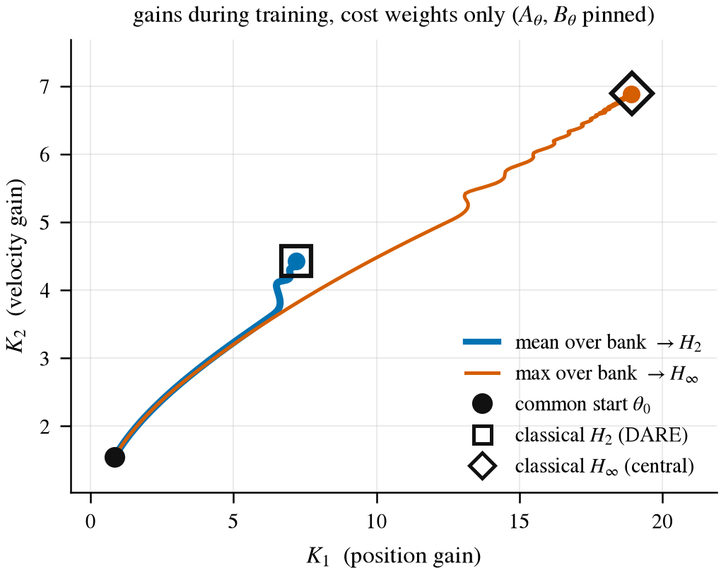
Gains during training: the mean objective converges to the classical H2 gain, the max objective to the classical H-infinity gain.
(a) Disturbance uncertainty. Averaging performance over disturbance frequencies yields an H2-type objective; taking the worst frequency yields an H∞-type objective. The learned gains approach the corresponding classical designs.
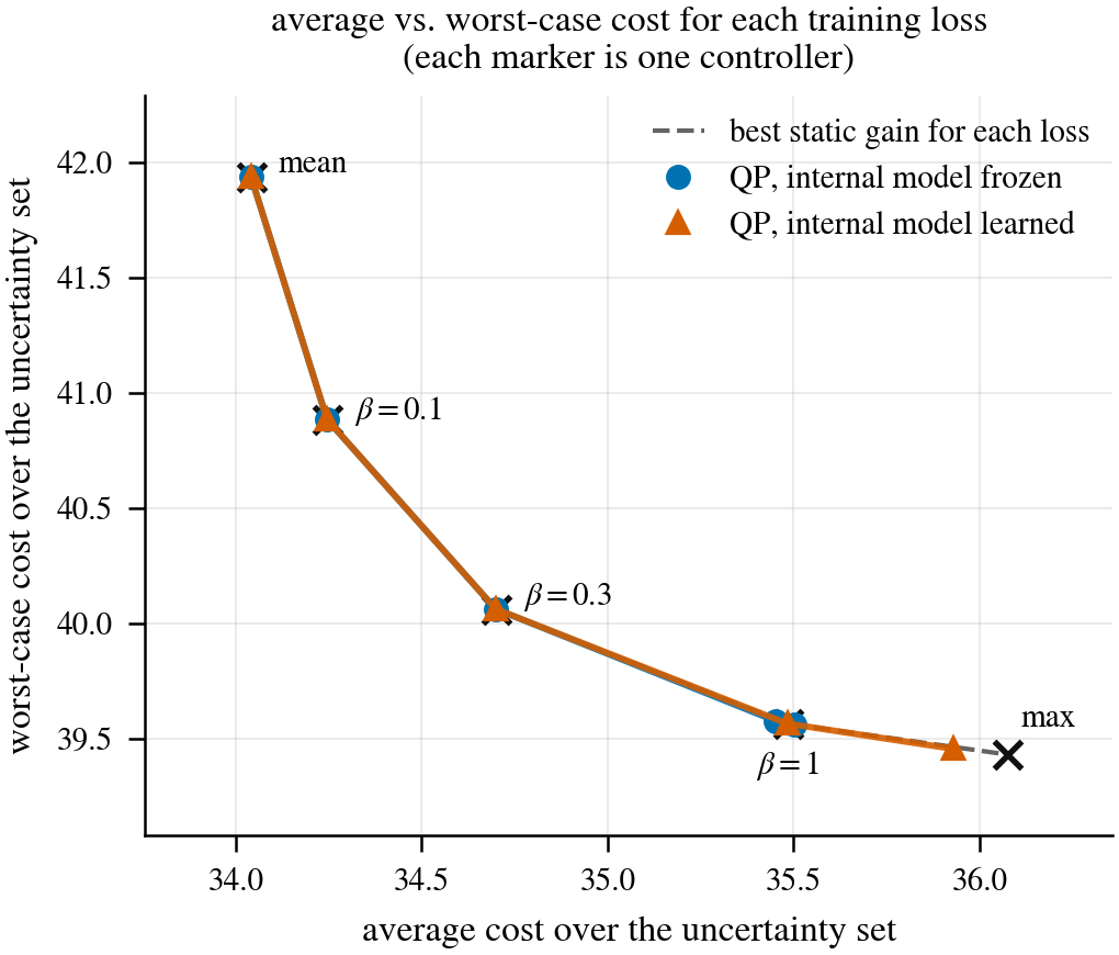
Average versus worst-case cost for controllers trained with increasing entropic risk parameter beta.
(b) Model uncertainty. Entropic risk continuously trades average-case performance for worst-case robustness as β increases.
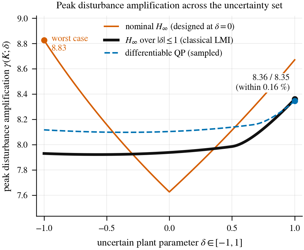
Peak disturbance amplification across the uncertain plant family for nominal H-infinity, classical LMI robust H-infinity, and the differentiable QP.
(c) Model + disturbance uncertainty. Taking the worst case over both plants and disturbances gives a sampled robust H∞ objective. The learned QP closely matches the classical robust design.

Robustness through domain randomization

Lunar lander with fuel slosh A lunar lander descending toward a landing target. The rigid body is modeled by the MPC. The fuel sloshing inside the tank is not in the MPC model and is randomized during training. Thrust and gimbal angle are the control inputs. Lunar lander with fuel slosh slosh is unmodeled by the MPC landing target Rigid body modeled by the MPC Fuel slosh not in the MPC model, randomized in training Thrust & gimbal control inputs
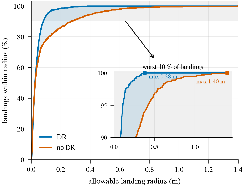
Percentage of 1,000 landings within a given radius, with and without domain randomization. Worst landing error: 0.38 m with DR, 1.40 m without.

Top left: lander model, with fuel slosh randomized during training. Bottom left: landing-error distribution across 1,000 vehicles. Right: final descent trajectories, with tighter clustering under domain randomization (DR).

Lunar lander with unmodeled fuel slosh

The MPC models only the lander's rigid-body dynamics, while the simulated plant also includes fuel slosh, modeled as a pendulum inside the tank, that the controller cannot see. During training, we randomize the slosh mass, pendulum length, and damping, and optimize the MPC cost parameters through closed-loop rollouts.

The resulting controller has the same online structure and computational cost as the nominal MPC, but is substantially more robust to slosh variation. Across 1,000 simulated vehicles, the worst landing error drops from 1.40 m to 0.38 m.

1,000simulated vehicles
0.38 mmax landing error, DR
1.40 mmax landing error, no DR

Hardware experiment

Crazyflie flight under strong crosswind

We deploy the full framework on a quadrotor flying through a 5 m/s crosswind. A disturbance observer estimates the persistent wind, while a trajectory-optimization QP computes the control commands.

The QP cost parameters and disturbance-observer gains are learned jointly from randomized closed-loop rollouts, rather than tuned separately by hand. Over five hardware trials, the learned policy rejects the disturbance faster and reaches lower steady-state position error than two manually tuned MPC baselines based on Bryson's rule.